In today's tutorial on Microsoft Excel 2007, we will look at the view tab. Using this Tab, you can control the layout and view of your Excel Workbook. This is especially important when you are done working on a spreadsheet and are finally ready to print it. So let us jump right into this and look at what the view tab in Microsoft Excel 2007 has to offer.
The View Tab split in two five Groups:
Workbook Views Group
Show/Hide Group
Zoom Group
Window Group
Macros Group
Workbook Views Group:
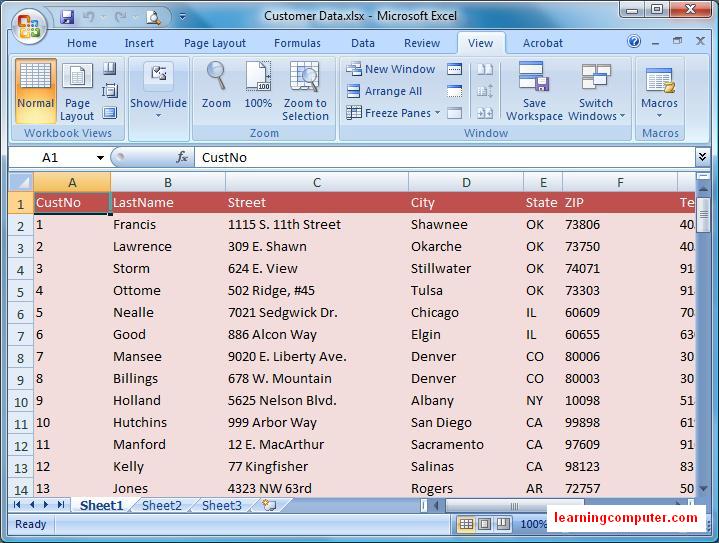
Using the Workbook Views Group of commands, you can view your Excel Workbook in different layouts. The Normal view is the default setting for Excel 2007. This is shown in the figure below. We are going to be using a Customer Workbook for today's practice. Using the Normal view you are able to view the rows and columns as you work on your spreadsheet.
|
 |
The second view on the Workbook Views tab is Page Layout. I find this particular view to be very helpful especially from a printing point of view.
Let us see what I am talking about. For your current Excel Workbook on customer data, go ahead and click the Page Layout command in the Ribbon. The effect of this action shown right below from our computer display. Notice that now you are able to see the header block, all the margins around the worksheet, the vertical and horizontal rulers and the column and row headings appear differently. If you were to print this work sheet, this is exactly what it would look like. Very nice!
|
 |
The next one is the Page Break Preview. This is again beneficial if you are trying to print an Excel sheet that spans multiple pages. This happens to be the case in our customer data worksheet. When I clicked on this command, my monitor displayed the following screen picture. Notice that I also got a dialog box letting me know that some information on page breaks. If you look closely at the customer data, you will see that page 1 includes five columns, then a dotted line, and finally we can see page 4 including the Zip and Telephone columns.
|
 |
Custom Views the next option will let you use a personalized view of your spreadsheet. You can even store this view so you can possibly use it on another workbook. The last view is Full Screen which will let you maximize the Excel sheet on your monitor display. Here's a screen shot of what I'm talking about. Notice that you do not see elements like the Ribbon, Scroll Bars, and Quick Access Toolbar etc. All you have is columns and rows of data so you can get more real estate on the computer.
|
 |
Show/Hide Group :
The next set of commands falls under Show/Hide group. These options are all listed as check boxes which can be turned on or off.
Let's play around with these commands next. For this exercise I'm going to switch back to Page Layout view first. This is what my data looks like before I do any make any changes
|
 |
First of all we are going to uncheck the Ruler option. This will go ahead and remove the horizontal and vertical rulers as you can see the effect in the following screen capture.
|
 |
Next try unchecking the Formula Bar option. Notice that it will remove the name box and the formula bar from your Excel Workbook as shown in the figure below.
|
 |
In the final option we will look at Headings check box which includes the row and column headings. In the following computer display, you will notice that we do not have any column and row headings.
|
 |
|
Zoom Group:
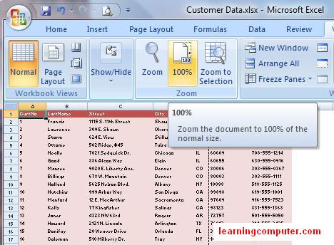
The next group we will look at is the Zoom Group. Using these commands you can control the area of your workbook that can be displayed on the computer monitor. The default is 100% which is what we have in the following screen capture. Also observe that we have switched back to the Normal view from the Page Layout for these steps.
|
 |
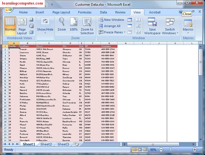
When you click on the Zoom command, you will get a new dialog box titled Zoom. Here you can direct the magnification level. It has a few preset options in addition to a custom choice where you can enter your own magnification level. For now go ahead and select 50% then click OK.
|
 |
After you click OK notice the effect of this action in the screen capture below. Now you can see all the fields related to your customer information. The size of the Headings has been adjusted to fit the Zooming level as well. If you look on the bottom right corner of the screen shot, you can also see the Zooming toolbar with the same value of 50%. This is another place where you can control the same functionality. |
 |
Let us go ahead and click on 100% which is the next command in the Zoom Group. This will convert the spreadsheet back to its normal magnification level.
|
 |
The last option is by far my favorite in this group. What if you wanted to highlight certain section of your Excel Workbook? No problem. Let us say that you wanted to see only 10 customers and the first four columns. You can select all the cells from A1 through D11 and then click on Zoom to Selection on the Ribbon.
The end result of this action shown in the screen display.
|
 |
Window Group :
Sometimes it is necessary to work on the same Excel sheet, however using multiple windows. The Window Group under the View Tab in Microsoft Excel will let you do just that. Let us take a look at these options next. Switch back to Normal view at 100% level and then click on New Window command on the Ribbon.
|
 |
This will open up a new Excel Workbook and title it Customer Data.xlsx:2. Shown right below in the screen capture of this step.
|
 |
Now that you have multiple copies of the same document, you are able to see them as the same time. Arrange All command can help you with this task. What you click on it, you will get the following dialog box as shown below. This is where you can choose how you would like to see the Windows. For now go ahead and choose Vertical and then click OK.
|
 |
|
The outcome of this action shown in the following screen capture. You now have the same Excel Workbook shown in a vertical fashion. This arrangement will let you view different sections of the same data at the same time, Sweet! Just realize that when you make changes in one, it will affect the other Excel Worksheet also.
|
 |
Moving onto the next command Freezing Panes which I think is a lifesaver that you are working with a complex spreadsheet. Using this great functionality, you can freeze particular rows and columns even as you walk around in your worksheet. Let us see in action next.
Our customer data sheet only has row headings. As such we do not need to worry about freezing columns. We would like to keep the Headings as we scrolled through my data. How can we do that? You can click on Freeze Panes and then choose Freeze Top Row from the drop down list.
We have included a screen shot of this step.
|
 |
Now as you move around in the Excel sheet, sideways or bottom, the column headings will stay frozen in place. For example in the following figure, we are looking at customer 46 yet we are still able to see the first row which includes column headings. This is Awesome!
|
 |
Let us take a look at a few more options under the Window Group. Using the Split command, you can essentially break your spreadsheet into different parts. This again can be useful when you need to look at different areas at the same time. You can select the cell where you would like the split to happen, for example we have chosen B32 as my Split Point. Notice our workbook now is split into four separate areas which we can view concurrently.
|
 |
When working with multiple Windows, the View Side by Side command will let you look at the data in a horizontal fashion. By default it also enables the Synchronous Scrolling feature, as you move up and down, the data in both windows will move in sync. You can disable this feature if you do not want synchronous scrolling feature.
|
 |
The final option we will look at is how to switch windows under the Window command. Once again if you have multiple copies of the same worksheet, you can use this command to toggle between windows back and forth. We have included a screen capture on our customer data spreadsheet. Notice that now we have a drop down which will let us switch to one of our open windows.
|
 |
| |

0 comments:
Post a Comment