Microsoft Excel 2007 Tutorial - Home Tab

Microsoft Excel 2007 Tutorial - Home Tab Home Tab in Microsoft Excel 2007 The Home Tab in Microsoft Excel 2007 has a lot of functionality for number crunching built right into it.  You can do things like formatting, alignment, inserting and deleting rows or columns, sorting and filtering numbers, applying styles and formatting effects, finding and replacing data and much more using the Tab. The Home Tab has the following groups that you can utilize: Clipboard Group Font Group Alignment Group Number Group Styles Group Cells Group Editing Group In order to understand some of these commands and functionality, we will be using a Grade Workbook from one of my prior classes. So let us jump right into it and start using the Home Tab in Excel 2007. Before we begin here is a screen shot of the student grades data that we will be using for practice. Clipboard Group: The first group is the Clipboard and it has commonly used commands like Cut, Copy and Paste.  Using these commands you can remove text from one area of your Microsoft Excel sheet to another.  When you use the Cut option, it removes the source text.  However when you use Copy option, it leaves the source text in place.  Using the Paste command, you can then insert the clipboard text into the new location.  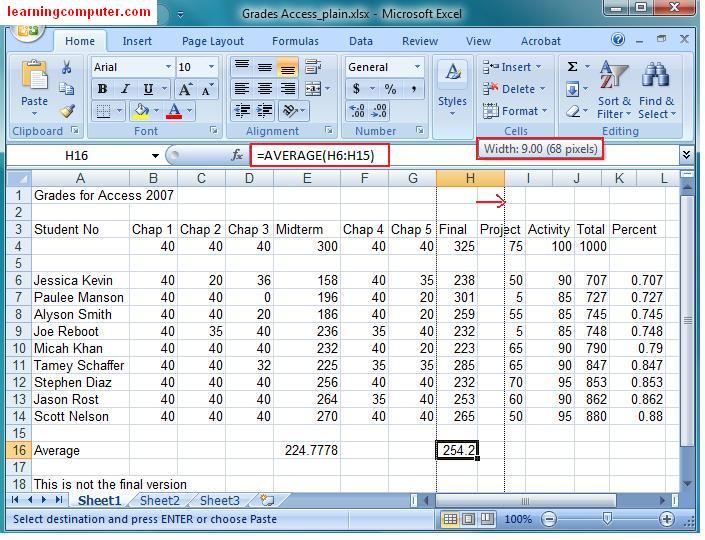Using these commands, you can also copy formulas and computed data from one area of the Excel worksheet to another.  In our case we have calculated the average of the Midterm test scores in cell E16.  We will cover how to compute the average in a later lesson. We would like to copy this formula and can use it for the Final test scores also.  How do we do that? Click on the cell E16 and you will, notice that in the formula bar (in red rectangle) we have the formula=AVERAGE(E6:E15) After you have selected the cell, click on copy command in the clipboard group. This is shown in the screen capture. Next we would like to use the same formula for the Final test scores in column H.  You can click in cell H16, and then click on Paste command from the clipboard group.  This will copy the average formula to cell H16 and compute the average for all the final test scores.  I also went ahead and changed the column width to nine characters or 68 pixels so we can see the average score a little clearly. We will cover changing column width in a different Excel tutorial. This is shown in the two screen shots below. Font Group: Moving onto the font group, here you can control the font properties of your text.  You can use drop down lists to change the font type and font size.  You can do actions like bold, italicize and underline text.  Let us say that for our Grades Excel Workbook, we need to change the size and font of text Grades for Access 2007.  Before I do this I need to adjust the first row height to something like 30 pixels.  The easiest way to adjust row height in Microsoft Excel is to select the row header [red circle], right click on the mouse and then select a row height.  These steps are illustrated in the figure below. I selected 30 pixels for my row height.  Next I went ahead and selected the text in cell A1 and then from Font type drop down chose Arial black.  In addition I used the font size dropdown in the Font group to choose size 14.  These two actions helped me emphasize the title text of my excel workbook.  I have included the screen shot for your review. 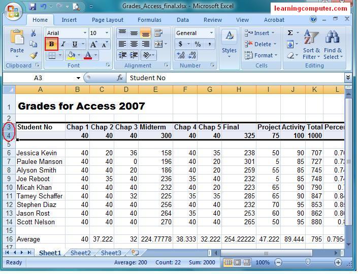We would also like to change rows 3 and 4 which include my class assignments, projects and tests headings to maybe Bold.  Let us show you the quickest way to do just that.  Using the left mouse you can highlight both the rows by selecting the row headers (red ovals).  Next you can click on the bold button on the font group to highlight the text.  This is shown in the figure below where the selected rows are now in Bold. 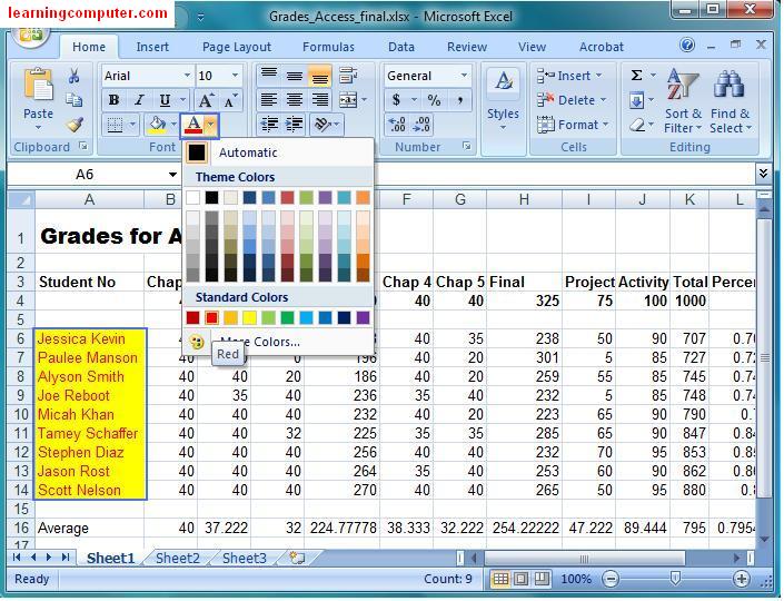One last thing I want to do using the font group in Excel 2007 is to change the background color and font color for my students names.  I want to use a yellow background and change the text to let's say red.  In order to achieve this, I need to select the student names from cells A6 through A14.  I can either use the mouse or the keyboard to do this.  I prefer to use the keyboard so I will click on a A6, hold down the Shift key while clicking on the down arrow one at a time until I have selected all the text. Next I will choose yellow from the background color drop down list.  This action is demonstrated below which changed the cells background to yellow. Next I will choose Red from the font color drop down to modify the actual text color. This is shown below in the screen capture.  As you can see our grade book is not looking so plain anymore.  So far we have changed font type, font size, bold option, background color and font color in Microsoft Excel 2007. 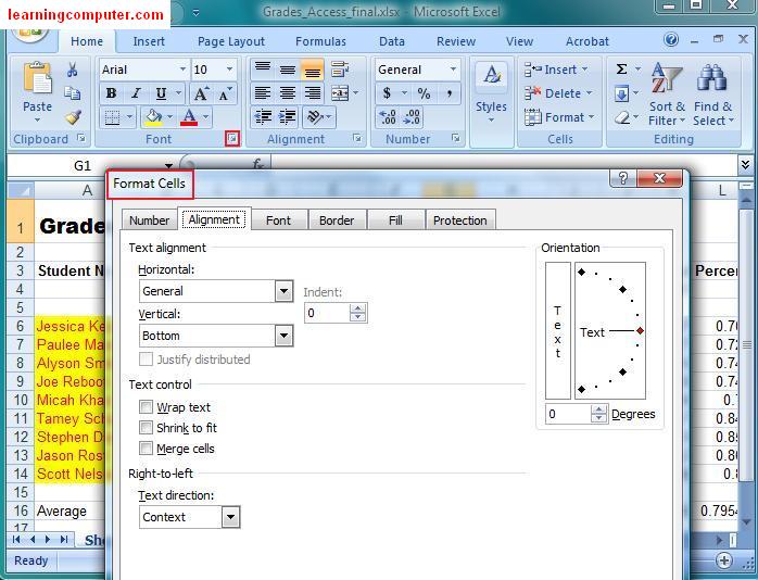If you still need more options to improve your font settings, you can certainly use the dialog box launcher shown by the small red square below.  This will launch the Format Cells dialog box which should look familiar from prior versions of Microsoft Excel. Alignment Group: We will move onto of the Alignment Group for the next set of exercises. Using the Alignment Group in Excel 2007, you can control the position and layout of text in your worksheet.  In my case, I would like to place all the assignments, project, midterm, final test scores in the middle of my cells. This is what needs to happen. Highlight all the text from cells B4 through J14, Next choose the Center command in the alignment tab under the Home Group in Excel 2007. This will affect the horizontal alignment and position all the scores in the center as shown below. Very Nice! Next I want to use Top Align option under the vertical alignment section for the text Grades for Access 2007.  Before I do this, I’m going to increase the first row height to 40 pixels.  After I have changed the row height, I will go ahead and select the text and then choose Center command from the vertical alignment area.  This is what it looks like in action. You can also use the Alignment Group to control some indentation in your excel 2007 sheet.  This functionality is commonly used in word processing like Word 2007, maybe not so much in a number crunching application.  We will skip over this option and show you the same effect by using the Merge & Center command. The Merge and Center command is a cool feature in Microsoft Excel 2007.  In the prior versions of Excel, I have struggled with this functionality, not anymore.  Lets us take a look at this feature.  Notice that the text for Grades for Access 2007 spans a few columns and is not in the middle of my worksheet.  I can easily achieve this by using the Merge and Center command.  I simply highlight the entire first row from the columns from A1 through L1, then select the Merge and Center command as visible in the figure below.  When I performed the above steps, it collapsed all columns into one, center alligned my text giving the heading a nice uniform feel that we desired. Here is what this looks like on my puter screen. The last vital option under the Allignment Tab is Wrap Text. This one is quite beneficial when you have to some long text in an Excel Sheet, however you would like to keep all the contents in one cell, no problem.  You will notice on the bottom of my excel sheet, I have text listed This is not the final version.  Notice that it spreads across three columns.  I would ideally like to wrap this text in one column.  I can easily do that using the Wrap Text option, this is what you need to do.  Highlight the text and then click on wrap text command button, Boom!  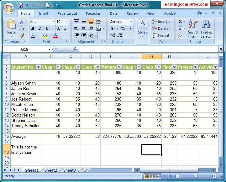As illustrated by the following figure, all the text has been wrapped into one cell, Perfect! 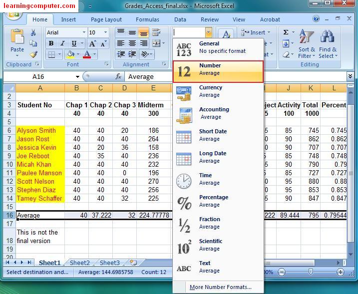Number Group: The next group that we will talk about is the Number group.  Here we have the option to change actual formatting for our data.  Let’s take a look at the average row which is 16 in the above screen shot. Observe that the decimal formatting is all jumbled up.  We would like to use the number formatting with 2nd place for decimal.  I will select the row 16, click on the dropdown list and then select Number.  This acion fixed the formatting issue for all of our Average scores. Similarly I would like to change the Percents in column L to a format where they are using the symbol instead of fractions. I will go ahead and highlight the data and then select the percent command under the Number group on the Home Tab in Microsoft Excel 2007. It went ahead and converted the percentage numbers to the correct format. The end result is visible right below in the two screen shots Styles Group: The styles group in Microsoft Excel 2007 has a lot of interesting options.  Let us experiment with these one at a time.  Here is a screen shot of the Styles Group. Using conditional formatting, you can highlight your data using a combination of color scales, icon sets, and data bars.  This will translate into a visual understanding off the underlying data that you are trying to analyze.  So in our case we would like to use conditional formatting to analyze students Total scores. We will first try the Data Bars option and then play around with the icon sets. First we need to increase the size of K column so we can accomodate all these cool analysis features. I will select the column header, right click and chose Column Width. In the next dialog box, I will type 10 for my width. This is displayed below. Now I am ready to experiment with conditional formatting.  I browse to the Styles group on the Home tab Microsoft Excel 2007.  From the drop down list, I will choose Conditional Formatting.  Next I will select Data Bars and then decide on Green Data bars as it is my favorite color.  I have highlighted the steps in the following screen capture. 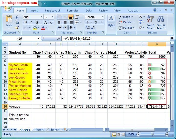In the following figure, You will notice that now in column K, we have different sized green data bars along with the total scores.  The size of the bar indicates the underlying data. For example student Jason Rost and Scott Nelson did quite well in our Access 2007 class.  On the flip side, Paulee Manson and Jessica Kevin did not do so hot.  As you can see, Conditional Formatting can give you a visual clues about your data, Sweet! I like this powerful conditional formatting feature Microsoft Excel 2007 so I will try one of the Icon Sets next.  What if I wanted to split my data into three groups, namely excellent, average and poor.  This time I will select Conditional Formatting, Icon sets and then choose 3 circled symbols.  This will yield the new breakdown as shown below.  We had really one student around the average score and the rest were either in the high or the low group. It gives definitely another perspective to my grade workbook. Before we move onto the next command, I would like to clear the formatting in my Excel 2007 sheet.  I will first highlight the data as shown below and then I will select clear command from the Editing group.  This will clear all the formatting that I had as shown below. This gives us a plain look before we experiment with Style galleries next. The Format as Table command will let you use one of the predefined, readymade out of the box styles in Microsoft Excel 2007.  A style is a combination of colors, font styles and graphical efeects that give your documents a professional and unique look.  Let’s play around with these next. I select the student data from cell A3 through L16. Next I click on Format as Table command in the Styles group. When I selected the drop down I was given an ellaborate list of gallery styles as shown below. In order to work with these styles, you can simply highlight the text and choose one of the many pre-defined styles. I went go ahead and chose the style hightlighted by the red rectangle below. This action applied a professional look to my student data as visible below. Notice that it also gave me filter capabilities so I can definitely put those to work if I desire. At this point I would like to do a Print Preview of how my Grades Workbook looks like. Here is the Print Preview output from my computer. I have a nice title followed by column headings and all the student scores look aligned and professional.   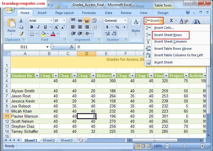Cells group: The Cells group is the next item that we are going to talk about.  Using the Insert command you can he can add cells, rows, columns and worksheets.  Let us say that we need to add a row after the student Paulee Manson.  I will select my mouse and then click on Insert Sheet Rows.  The Insert options are shown in the screen shot below. Please note that we will cover insert and delete coneclpts in our video training so be sure to check those out. Let’s assume what we did in the previous stpe was a mistake and we would like to undo that action.  You can easily do that by using the delete command.  Using the Delete commands under the Cells group, you can delete cells, rows, columns and the sheets. Here are the possible Delete options. The last option is Format command in the Cells group in Microsoft Excel 2007.  This option has a host of menu options to choose from.  You can do things like to adjust row height/column width, unhide/hide columns and rows and finally use the Auto Fit functionality.  I would like to use auto fit on all my columns.  I will highlight them, click on the format drop down and then select Autofit Column Width.  Here is a screen capture of what this looks like. Editing group The last group we want to look at is the Editing group on Microsoft Excel Home tab. The two commands that we will talk about here are sort and filter plus find and select.  The first one will let you sort data in an ascending or descending order easily.  If you want to do asending order, you can select sort from smallest to largest.  Conversely if you want to use descending order, you can sort from largest to smallestr.  Next you are going to show you the custom sort. I would like to get a glimpse of how all the students did overall.  I could select the underlying data which is in cells B6 through K14.  Next select custom sort from the Sort and Filter command. This will invoke the sort dialog box as shown below. I will choose column K (Total) and then select Smallest to Largest under the order.  When I did this, I was able to see Jessica Kevin scored the lowest and Scott Nelsen scored the highest.  This is displayed in the next two screen captures below. 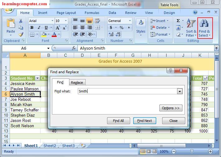Finally the last command that we will take a look at is Find and Select.  In our example this dataset is quite small, but let’s try this action anyway.  Say we were looking for someone with a last name Smith.  I would choose Find from the dropdown under Find and Select.  This will popup the Find and Replace dialog box as shown below. I will enter Smith and in Find What and then click Find next.  Notice that it was able to find a student with that name in cell A6. This concludes the tutorial on Home Tab in Microsoft Excel 2007.

Posted in: How to, MS Excel, Tips and Tricks, Tutorials